44 data labels excel pie chart
Microsoft Excel Tutorials: Add Data Labels to a Pie Chart To add the numbers from our E column (the viewing figures), left click on the pie chart itself to select it: The chart is selected when you can see all those blue circles surrounding it. Now right click the chart. You should get the following menu: From the menu, select Add Data Labels. New data labels will then appear on your chart: How to Edit Pie Chart in Excel (All Possible Modifications) How to Edit Pie Chart in Excel 1. Change Chart Color 2. Change Background Color 3. Change Font of Pie Chart 4. Change Chart Border 5. Resize Pie Chart 6. Change Chart Title Position 7. Change Data Labels Position 8. Show Percentage on Data Labels 9. Change Pie Chart's Legend Position 10. Edit Pie Chart Using Switch Row/Column Button 11.
Change the format of data labels in a chart To get there, after adding your data labels, select the data label to format, and then click Chart Elements > Data Labels > More Options. To go to the appropriate area, click one of the four icons ( Fill & Line, Effects, Size & Properties ( Layout & Properties in Outlook or Word), or Label Options) shown here.
Data labels excel pie chart
excel - Pie Chart VBA DataLabel Formatting - Stack Overflow sub updatechartformat () with activeworkbook.sheets ("mhfa summary").chartobjects ("chart 4").activate with activechart.seriescollection (1).datalabels _ .showpercentage = true with activechart.seriescollection (1).datalabels _ .separator = "" & chr (10) & "" end with end with end with with activeworkbook.sheets ("mhfa … excel - How to not display labels in pie chart that are 0% - Stack Overflow Generate a new column with the following formula: =IF (B2=0,"",A2) Then right click on the labels and choose "Format Data Labels". Check "Value From Cells", choosing the column with the formula and percentage of the Label Options. Under Label Options -> Number -> Category, choose "Custom". Under Format Code, enter the following: Display data point labels outside a pie chart in a paginated report ... Create a pie chart and display the data labels. Open the Properties pane. On the design surface, click on the pie itself to display the Category properties in the Properties pane. Expand the CustomAttributes node. A list of attributes for the pie chart is displayed. Set the PieLabelStyle property to Outside. Set the PieLineColor property to Black.
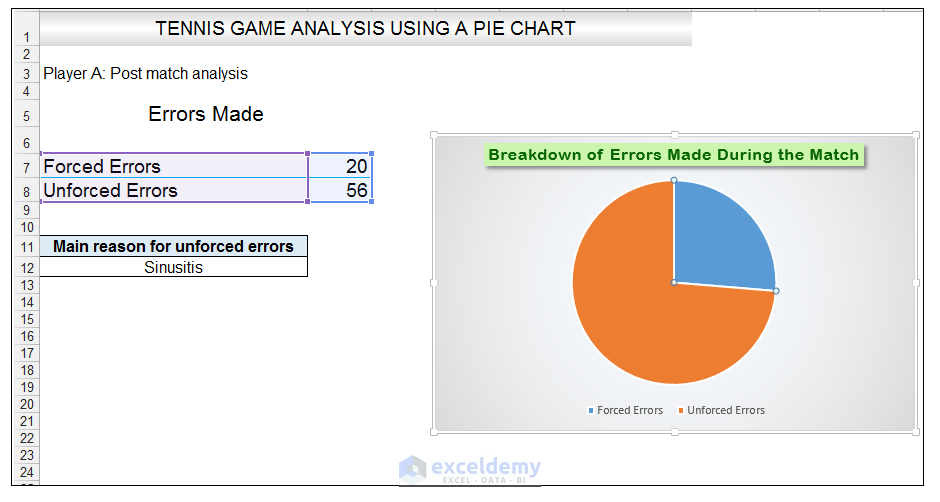
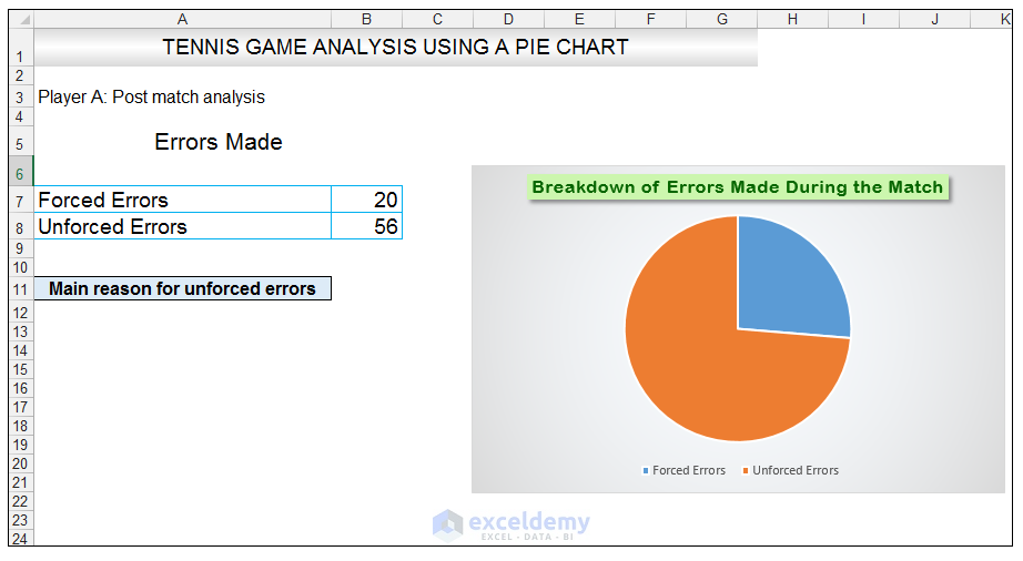
Data labels excel pie chart. How to Make a Pie Chart in Excel & Add Rich Data Labels to The Chart! Creating and formatting the Pie Chart 1) Select the data. 2) Go to Insert> Charts> click on the drop-down arrow next to Pie Chart and under 2-D Pie, select the Pie Chart, shown below. 3) Chang the chart title to Breakdown of Errors Made During the Match, by clicking on it and typing the new title. Inserting Data Label in the Color Legend of a pie chart Inserting Data Label in the Color Legend of a pie chart. Hi, I am trying to insert data labels (percentages) as part of the side colored legend, rather than on the pie chart itself, as displayed on the image below. Does Excel offer that option and if so, how can i go about it? How to Make a Pie Chart in Excel (Only Guide You Need) To add labels to the slices of the pie chart do the following. 1 st select the pie chart and press on to the "+" shaped button which is actually the Chart Elements option Then put a tick mark on the Data Labels You will see that the data labels are inserted into the slices of your pie chart. How to create a pie chart in Microsoft Excel Remember that when a user changes the pie chart data, it will automatically update. Create basic pie chart. You can create pie charts in two different ways and both start by selecting cells. Be sure to select only the cells you want to convert into a chart. Method 1. Select the cells, right-click the selected group and select Quick Analysis ...
How to Create and Format a Pie Chart in Excel - Lifewire Select the plot area of the pie chart. Select a slice of the pie chart to surround the slice with small blue highlight dots. Drag the slice away from the pie chart to explode it. To reposition a data label, select the data label to select all data labels. Select the data label you want to move and drag it to the desired location. pie chart - Hide a range of data labels in 'pie of pie' in Excel ... First format the second pie so that each slice has no fill (becomes invisible), to speed this up just set the first slice to no fill and then highlight each slice and select F4 to repeat last action. Next select any slice from the main chart and hit CTRL+1 to bring up the Series Option window, here set the gap width to 0% (this will centre the ... excel - Positioning data labels in pie chart - Stack Overflow Sub tester () Dim se As Series Set se = Totalt.ChartObjects ("Inosa gule").Chart.SeriesCollection ("Grøn pil") se.ApplyDataLabels With se.DataLabels .NumberFormat = "0,0 %" With .Format.Fill .ForeColor.RGB = RGB (255, 255, 255) .Transparency = 0.15 End With .Position = xlLabelPositionCenter End With End Sub Adding data labels to a pie chart - Excel General - OzGrid Re: Adding data labels to a pie chart. Thanks again, norie. Really appreciate the help. I tried recording a macro while doing it manually (before my first post). But it didn't record anything about labels, much less making them bold.
Office: Display Data Labels in a Pie Chart - Tech-Recipes If you have not inserted a chart yet, go to the Insert tab on the ribbon, and click the Chart option. 3. In the Chart window, choose the Pie chart option from the list on the left. Next, choose the type of pie chart you want on the right side. 4. Once the chart is inserted into the document, you will notice that there are no data labels. Move data labels - support.microsoft.com Right-click the selection > Chart Elements > Data Labels arrow, and select the placement option you want. Different options are available for different chart types. For example, you can place data labels outside of the data points in a pie chart but not in a column chart. Pie of Pie Chart in Excel - Inserting, Customizing, Formatting Inserting a Pie of Pie Chart. Let us say we have the sales of different items of a bakery. Below is the data:-. To insert a Pie of Pie chart:-. Select the data range A1:B7. Enter in the Insert Tab. Select the Pie button, in the charts group. Select Pie of Pie chart in the 2D chart section. How to add data labels from different column in an Excel chart? Please do as follows: 1. Right click the data series in the chart, and select Add Data Labels > Add Data Labels from the context menu to add data labels. 2. Right click the data series, and select Format Data Labels from the context menu. 3.
How to Create Excel Pie Charts & Add Rich Data Labels to The Chart!
Multiple data labels (in separate locations on chart) You can use the Up/Down arrows to move through chart elements in order to select the second pie. Or use the drop down on the charting toolbar to select the 2nd series Attached Files 819208a.xlsx (77.9 KB, 401 views) Download Register To Reply 08-16-2013, 05:58 AM #6 petesurfer Registered User Join Date 04-16-2013 Location London, England

32 How To Label Pie Chart - Labels 2021
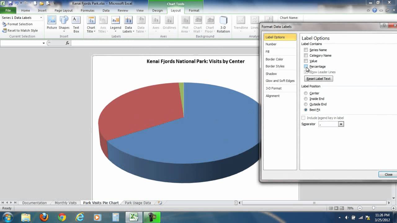
Excel 2010 pie chart data labels in case of "Best Fit" Based on my tested in Excel 2010, the data labels in the "Inside" or "Outside" is based on the data source. If the gap between the data is big, the data labels and leader lines is "outside" the chart. and leader lines is "inside" the chart. Regards, George ZhaoTechNet Community Support Friday, July 25, 2014 6:31 AM
How to Create Excel Pie Charts & Add Rich Data Labels to The Chart!
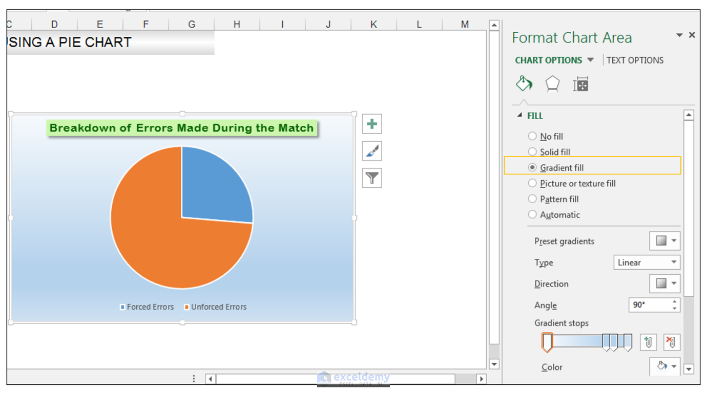
Create a Pie Chart in Excel (In Easy Steps) Create the pie chart (repeat steps 2-3). 7. Click the legend at the bottom and press Delete. 8. Select the pie chart. 9. Click the + button on the right side of the chart and click the check box next to Data Labels. 10. Click the paintbrush icon on the right side of the chart and change the color scheme of the pie chart.

How to Make Bubble Charts | FlowingData
Pie Chart in Excel - Inserting, Formatting, Filters, Data Labels The total of percentages of the data point in the pie chart would be 100% in all cases. Consequently, we can add Data Labels on the pie chart to show the numerical values of the data points. We can use Pie Charts to represent: ratio of population of male and female of a country. proportion of online/offline payment modes of a local car rental ...

Creating Pie Chart and Adding/Formatting Data Labels (E... | Doovi
Chart Legend / Data Labels In Pie Chart | MrExcel Message Board Jun 6, 2009. #3. Add the data labels. Then, right click on any data label to select all the data labels for that series and select Format Data Labels... From the Label Options tab, in the Label Contains section, select the 'Series Name' checkbox. The above applies to Excel 2007. Excel 2003 supports the same capability though the dialog box ...
How to Make a Pie Chart in Excel & Add Rich Data Labels to The Chart!
Edit titles or data labels in a chart - support.microsoft.com On a chart, click one time or two times on the data label that you want to link to a corresponding worksheet cell. The first click selects the data labels for the whole data series, and the second click selects the individual data label. Right-click the data label, and then click Format Data Label or Format Data Labels.

How to Make Pie Charts and Graphs in Excel - BSUPERIOR
How to display leader lines in pie chart in Excel? - ExtendOffice To display leader lines in pie chart, you just need to check an option then drag the labels out. 1. Click at the chart, and right click to select Format Data Labels from context menu. 2. In the popping Format Data Labels dialog/pane, check Show Leader Lines in the Label Options section. See screenshot: 3.

34 Tableau Pie Chart Percentage Label - Labels Database 2020
Add or remove data labels in a chart - support.microsoft.com Click the data series or chart. To label one data point, after clicking the series, click that data point. In the upper right corner, next to the chart, click Add Chart Element > Data Labels. To change the location, click the arrow, and choose an option. If you want to show your data label inside a text bubble shape, click Data Callout.

Pie Chart - PK: An Excel Expert
Formatting data labels and printing pie charts on Excel for Mac 2019 ... Here's a work around I found for printing pie charts. Still can't find a solution for formatting the data labels. 1. When printing a pie chart from Excel for mac 2019, MS instructions are to select the chart only, on the worksheet > file > print. Excel is supposed to print the chart only (not the data ) and automatically fit it onto one page.
Chart Elements :: Hour 12. Adding a Chart :: Part III: Interactive Data Makes Your Worksheet ...
Pie Chart in Excel | How to Create Pie Chart - EDUCBA Pie Chart in Excel Pie Chart in Excel is used for showing the completion or main contribution of different segments out of 100%. It is like each value represents the portion of the Slice from the total complete Pie. For Example, we have 4 values A, B, C and D.
Creating a 3D Pie Chart in Excel Vid.wmv - YouTube
Display data point labels outside a pie chart in a paginated report ... Create a pie chart and display the data labels. Open the Properties pane. On the design surface, click on the pie itself to display the Category properties in the Properties pane. Expand the CustomAttributes node. A list of attributes for the pie chart is displayed. Set the PieLabelStyle property to Outside. Set the PieLineColor property to Black.

how to label pie chart in excel - Labels 2021
excel - How to not display labels in pie chart that are 0% - Stack Overflow Generate a new column with the following formula: =IF (B2=0,"",A2) Then right click on the labels and choose "Format Data Labels". Check "Value From Cells", choosing the column with the formula and percentage of the Label Options. Under Label Options -> Number -> Category, choose "Custom". Under Format Code, enter the following:

How to Make a Pie Chart in Excel & Add Rich Data Labels to The Chart!
excel - Pie Chart VBA DataLabel Formatting - Stack Overflow sub updatechartformat () with activeworkbook.sheets ("mhfa summary").chartobjects ("chart 4").activate with activechart.seriescollection (1).datalabels _ .showpercentage = true with activechart.seriescollection (1).datalabels _ .separator = "" & chr (10) & "" end with end with end with with activeworkbook.sheets ("mhfa …

How to Create a Pie Chart in Excel | Smartsheet

33 How To Label A Pie Chart In Excel - Labels 2021
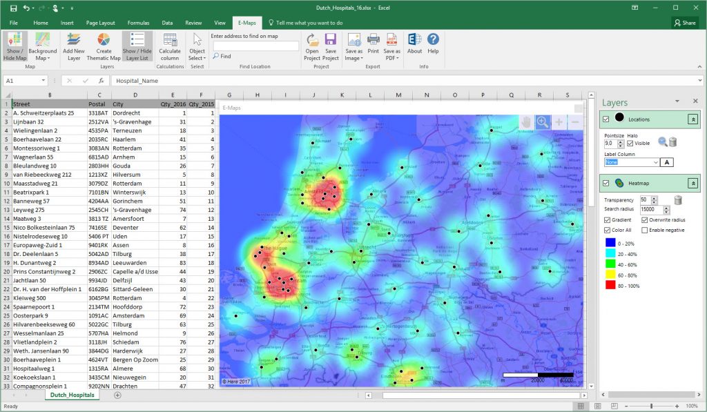
Adjustable colours and ranges in heatmap - Excel E-Maps

Part 2—Explore Biodiversity Using A Forest Inventory Growth (FIG) Dataset from Maine

Science + Technology: Student Technology Usage Survey and Podcast
Post a Comment for "44 data labels excel pie chart"